Stage to Image¶

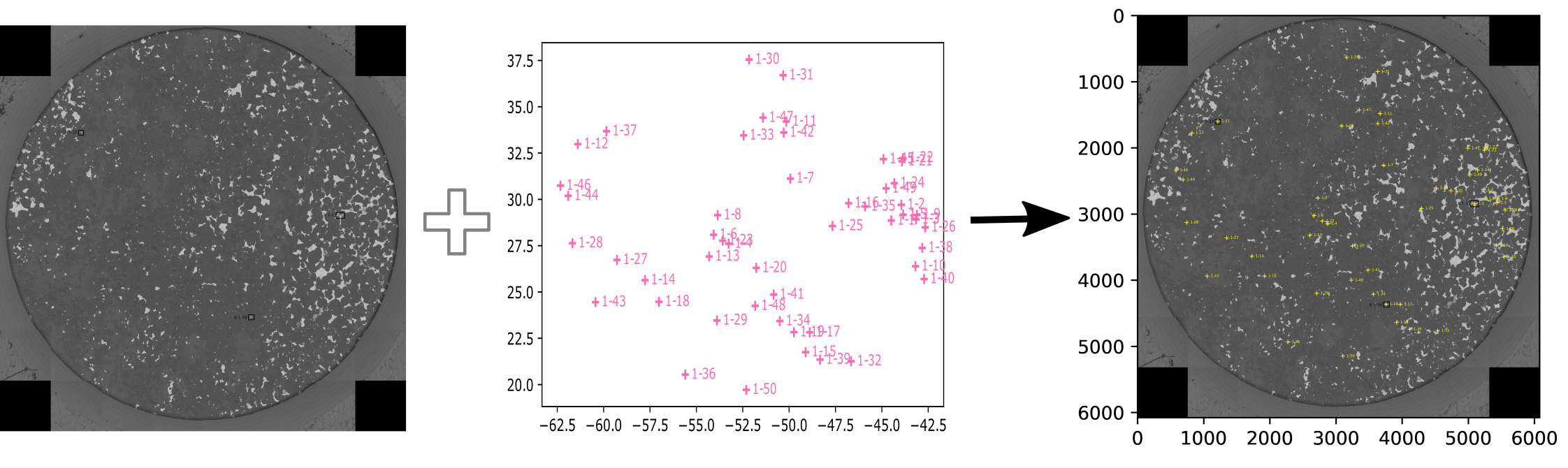
This is a simple workflow example involving converting points from one stage coordinate system to display on a large image. This helps to visualise where the analysis were collected and gives context to the anaysis.

INPUT:

.csv - a list of X,Y coordinates with spotnames + more than 3 reference points
large image with locations of more than 3 reference points

OUTPUT:

image with points labelled

e.g. We have been using the workflow to visualise the microanalysis points from SEM on large reflected light images

Input and output can be easily changed for your purposes see the contributions page for more information on how to contribute.

Step 1: Acquire image¶

collect an image of the sample

Remember to highlight 3 regions or more for registration points

Step 2: Calibrate and Transform the points between the the image and the stage¶

Import your CSV file with analysed points

specify your >3 reference coordinates using the autopew interactive interface

specify the stage Coordinates of these reference points

Use autopew to transform all stage coordinates. See the example code below:

Note that the calibration of this transform involves a least-squares process to find the optimal transformation, such that adding more calibration points can help avoid minor inaccuracies in adding points.

from pathlib import Path
import numpy as np
import matplotlib.pyplot as plt
from PIL import Image
from autopew import Pew
from autopew.workflow import pick_points

imagepath = Path("./../../source/_static/") / "SEM_RefPoints.png"

# %% REFERENCE POINTS ------------------------------------------------------------
#these are the known locations of the reference points in the laser coordinate system
laser_reference_coords =np.array([[45633,9098],  #R1-ccp55
                                  [56683,17876], #R2-ccp33
                                  [43301,16082], #R3-ccp38
                                  [42096,5137]]) #R4-pn25

#pick the reference points on the image
img_reference_coords = pick_points(imagepath)

# %% TRANSFORM laser to pixels ---------------------------------------------------------------
points = (Pew(laser_reference_coords,
              img_reference_coords)
              .load_samples('Samples.csv'))

Step 4: Overlay the image and the points¶

Export an image containing labelled point overlay over image

# FIND THE PIXEL SIZE OF THE IMAGE
img = Image.open(imagepath)
# get the image's width and height in pixels
width, height = img.size

fig, ax = plt.subplots()
ax.scatter(points.transformed['x'], points.transformed['y'],facecolors='none', edgecolors='y', marker="o",zorder=1,s=6,linewidth=.3)

for i, df in enumerate(points.transformed['name']):
  ax.annotate(df, (points.transformed.x[i], points.transformed.y[i]),
              xytext=(2, 0), textcoords='offset points',
              horizontalalignment='left', verticalalignment='center',
              size=4, color='yellow',
              zorder=1)
ax.set(xlim=(0, width), ylim=(0, height))

plt.imshow(img, zorder=0)
ax.invert_yaxis()#image invert so it is the same up direction as import.

plt.tight_layout()
plt.show()
#fig.savefig('Export_image.png', transparent=True, dpi=800)